Stochastic Model of Aircraft Trajectories
Departing aircraft $i$ is parked at a gate. Upon receiving the push back clearance, a tug (operated by ground crew) pushes back the aircraft from the gate. At the end of the push back procedure, the aircraft stops and the tug disengages. This stop period lasts for some time during which the pilot goes through a checklist and then starts the aircraft engine(s). When ready, the pilot requests taxi approval, and after the approval, the aircraft taxies until arriving at time $t_i$ at the terminal node (P1), as shown in the Figure below. During the departing maneuvers, the duration of the trajectory, the transitions over the motion phases, and the trajectory path are determined by human operators and are stochastic in nature.

Arriving aircraft $i$ begins its trajectory at the initial node (P2), see Figure below. After being released from the initial node at time $t_i$, the aircraft taxies to the assigned gate. During the arriving maneuvers the duration of the trajectory and the trajectory path are considered to be stochastic.

The ramp area is defined as the aircraft moving area between the taxiway spots and the gates. For both departures and arrivals, the locations of the initial node (P2) and the terminal node (P1) in our model define a boundary between the domain where trajectories are well-defined and the domain where trajectories are stochastic.
We collect data influenced by a human operator and use the data to fit parameters of our stochastic model of aircraft trajectories. Once the model is defined we use it to sample a large number of realistic trajectories. The sampled trajectories are used to build a probabilistic measure of conflict within the ramp area. After generating the measure of conflict, we calculate the necessary separation constraints in time among aircraft that ensure conflict free trajectories within the ramp area. A single ramp area departure trajectory for aircraft $i$ is described by five discrete states $q$, $q = 0, 1, .. , 4.$ Each discrete state is defined by the continuous time evolution of the aircraft $i$'s position and heading angle described by $x^i$, $y^i$ coordinates and $\theta^i$, respectively:
For $q=0$ (gate), $q=2$ (stop), $q=4$ (terminal node): \begin{align} dx^i =0, \,\, dy^i = 0, \,\, d \theta^i =0 \end{align} For $q=1$ (push back): \begin{align} dx^i =-v_P^i \cos ( \theta^i) dt, \,\, dy^i = -v_P^i \sin( \theta^i) dt, \,\, d \theta^i =- \frac{v_P^i}{R^i} dt \end{align}where $R^i$ is the radius of the circle of curvature that aircraft $i$ is pushing back along and $v_P^i$ is the push back velocity.
For $q=3$ (taxi): \begin{align} dx^i =v_T^i \cos ( \theta^i) dt, \,\, dy^i = v_T^i \sin( \theta^i) dt, \,\, d \theta^i = \sigma^i dW^i \end{align}where $dW^i$ is an increment of a unit intensity Wiener process, $\sigma^i$ is a scaling factor for the intensity of the variations in the heading angle $ \theta^i$, and $v_T^i$ is the forward taxi velocity for aircraft $i$. In a similar fashion we can define the three discrete states $q$ defined by the continuous time evolution for an arriving aircraft $i$ (q=0, 1, 2):
For $q=0$ (initial node), $q=2$ (gate) \begin{align} dx^i =0, \,\, dy^i = 0, \,\, d \theta^i =0 \end{align} For $q=1$ (taxi): \begin{align} dx^i =v^i \cos ( \theta^i) dt, \,\, dy^i = v^i \sin( \theta^i) dt, \,\, d \theta^i = \sigma^i dW^i \end{align}
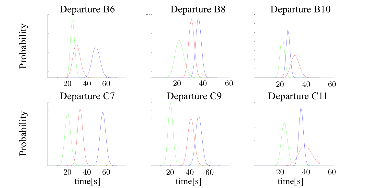
Transitions between discrete states are considered to be stochastic. In order to simulate a single departure trajectory, we sample the times for states $q=1,2,3$ from the gamma distribution that was fitted to the robot experiment data. Transitions between the states are defined by the values of the sampled times. In general, the times that we sample for the discrete states will never match exactly between two unique trajectories. For the set of successful samples, this temporal uncertainty will produce a distribution over the trajectory duration. This distribution in trajectory duration is directly influenced by the human operator.

In addition to the initial conditions and parameters, we also define a terminal condition the trajectory sample must satisfy. Given that our trajectories are described by an uncontrolled stochastic processes, in general we do not expect the departure (arrival) samples to terminate at the terminal node (gate). However, if we sample enough departure (arrival) trajectories, we do expect for some samples to arrive at the terminal node (gate) as desired. Conditioning the trajectories to terminate within the goal region provides a set of feasible ramp area departure (arrival) trajectories that terminate (initiate) their trajectory at time $t_i$.
After sampling trajectories we estimate the probability density function for trajectory duration of aircraft $i$ in the absence of any other aircraft in the ramp area. We refer to this type of distribution as $natural$ since the aircraft is unimpeded. We are interested in computing push back windows for aircraft $i$ such that the aircraft arrives at the terminal node at a scheduled time $t_i$. Therefore, we enforce a terminal condition in time for the sampled trajectories and this generates a distribution for the push back time. In addition, enforcing this terminal condition in time provides us with a set of departing trajectories that all enter the FAA controlled taxiway via the taxiway spot at the same time, as required by the optimal schedule.
Sampled trajectories within center alley at CLT airport:

Sampled departure trajectories from gate B6 at CLT airport: