Table of Contents
Computer Science: Artificial Intelligence
Introductions to the Class
- thoughtfulplay.com
- What is each student's favorite game?
- Favorite Subject?
Introduction to Computers
- What do Humans do better than Computers?
- Sudokubot: https://www.youtube.com/watch?v=Mp8Y2yjV4fU
- Pancakebot: https://www.youtube.com/watch?v=BEJZDng1UBs
- Catching Robot: https://www.youtube.com/watch?v=M413lLWvrbI
- Looking at Code
- Neo sees code: https://www.youtube.com/watch?v=SdkdQtlF-RU
Arduino
Animations and Computer Graphics
- Jared Counts: https://www.youtube.com/watch?v=TQJbJVCMIH8
Artificial Intelligence
Car
- Dystopian Future: https://www.youtube.com/watch?v=h1BQPV-iCkU
Where do we get our measure of intelligence?
- Intellivator: https://www.youtube.com/watch?v=k2Cev3Ft4zg
- Cleverbot: https://www.youtube.com/watch?v=WnzlbyTZsQY
- Argument Champion
- 20Q and Akinator
Alan Turing
- Imitation Game: https://www.youtube.com/watch?v=S5CjKEFb-sM
- Evie: http://www.existor.com/
- PromWeek
Algorithms
Assignment
Introduction to Computer Graphics
First, go to http://openprocessing.org
(if you want to save all of your work for when you go back home, PLEASE sign up for an account)
Introduction to Processing (credit: DMA)
Most intro programming classes begin with text-based exercises and basic command line prompts. With Processing, we will be learning to program visually through manipulating images. Processing syntax is very similar to Java, a good understanding of the basics of Processing will give you a head start on the Java applet and game design sections over the rest of the week.
Why learn Processing?
The Processing environment is actually written in Java! Processing code is translated(compiled) into Java and is run as a Java program.
Starting with Processing allows you to have a basic graphics library at your disposal without worrying about more advanced Java concepts and object-oriented programming.
The goal of this lesson is to introduce you to programming and get you comfortable with drawing shapes through code. You will also learn about tracking mouse positions in order to make your graphics more interactive.
1. Your first Processing application
Line Drawings
Let’s get to drawing with code! Open up a new Processing sketch and type the following into the text editor area:
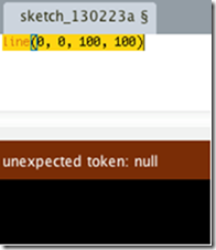
line (0, 0, 100, 100);
This is our first function (more on functions later)! The line function is surrounded by brackets ( ) containing 4 numbers, separated by commas. The values within the brackets are called parameters (Provide a definition of a function and parameters, simple explanation).
Notice the semi-colon (;) at the end of the statement. The semi-colon is a very important part of Java syntax, it tells the compiler that you have finished your statement. Syntax is an important part of programming (specificity of language).
Programming languages are precise and will not run if you forget a semicolon or give your function the incorrect number or type of arguments. If you receive an error message while trying to run your application, don’t panic! The compiler will catch any errors in your code and offer suggestions to help fix the problem. This is an invaluable resource as you progress through the lesson material. Even professional programmers make errors quite often and that is why it is important to test your code often!
Let’s add another line:
line (100, 0, 0, 100);
Try running the code again.
We have created an X shape across the screen by constructing two lines, but how exactly does this work?
The numbers in the line function represent coordinate positions. You may have learned in Math class that coordinates are represented by two numbers in brackets representing the X (horizontal) and Y (vertical) position of a point. The line function takes two coordinates points as arguments and draws a line between the two points.
The coordinate system in Processing starts from the upper left hand corner (position 0, 0). This means that as your x value increases, the point moves RIGHT, and similarly, as your y value increases, your coordinate will move DOWN. This is important to remember as it will determine the placement of all the elements coded in your application.
By default, Processing runs on a 100 x 100 pixel window (we’ll see in a bit how to adjust the screen size). Our two lines are represented by two sets of coordinate points. Our first line function draws a line from point (0, 0) to point (100, 100) and the second line draws a line from point (0, 100) to point (0, 100).
Rectangles and Circles (Ellipses)
Here is the code we use to draw rectangles and ellipses. We will continue to build on top of the line drawings we constructed during the previous section.
rect( x_position, y_position, width, height)
*Remember that X and Y positions start at the upper left hand corner, position (0, 0).
Let’s make some rectangles! Type this code below your line code:
rectMode(CENTER);
rect(50, 50, 50, 50);
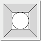
Our rectangle will be drawn centered at position (50, 50) with a width of 50 and a height of 50. This effectively makes a square.
Run the code. You should see a square appear at the center of your lines. Notice that the rectangle is drawn on top of the lines. It is important to note that Processing draws images in the order that they are written in the code. If you place the rectangle code before the line code, the lines will appear on top of the rectangles.
Next up, let’s draw an ellipse!
The arguments (parameters) for drawing an ellipse are very similar to that of a rectangle:
ellipse (x_position, y_position, width, height)
Type this code below your rectangle code:
ellipseMode(CENTER);
ellipse(50, 50, 50, 50);
Run this code again, and you should see a circle appear inside of your rectangle.
The code ellipseMode(CENTER) and rectMode(CENTER) mean that our coordinate positions (the first and second parameters of the function) for rectangle and ellipses are based on the center of our shape.
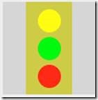
2. Make a traffic light!
Let’s do an exercise to test your understanding of coordinate positioning.
The code lines that start with are comments. They do not change the functionality of a program, but are used to provider helpful hints to the programmer. Comments are an essential part of writing good code. Effective comments let you understand what a program does before running it. This is especially useful if you plan on sharing your codes with others. this is a comment! tell me how your program works! /* This is a multi-lined comment. I could go on forever. Don’t forget to close me! */
Let’s take a look at the green light ellipse code first.
ellipse (10, 20, 25, 25);
The vertical positioning looks fine (the green light belongs at the top), but the horizontal positioning is slightly off. Recall that increases in our X position (the first argument of ellipse) will move our circle to the right.
Let’s increase the value of x to 50:
ellipse (50, 20, 25, 25);
Run your application to double check your work. That position looks about right!
Moving on to the yellow light. The horizontal positioning looks find but the yellow light is too far down our traffic light.
To move the yellow light up, we need to decrease the y position value from its current value of 70. Let’s change it to 50:
ellipse(50, 50, 25, 25);
Much better! The red light is not positioned correctly at all, and is almost falling off of the screen. Can you guess what the correct x position is for the red light? By looking at our two previous ellipses, we can get the correct x position value of 50. When trying to adjust parts of your program, it is always useful to look back at the code you have already written, it usually contains hints about how to fix your current line of code!
ellipse(50, 100, 25, 25);
What about the vertical position of the red light? Try decreasing the value of the y position by 5 or 10 and run the code to see the difference. The correct spacing will be around 80.
The final positioning of the red light should be something similar to this:
ellipse(50, 80, 25, 25);
Run your code again to double check your work, you should see a nicely organized traffic light!
Notice that the difference between the Y position of the green light is
50 – 20 = 30 and similarly, the difference between the Y position of the yellow light and the red light is 80-50 = 30. By comparing the values of the position of our shapes using simple math, we can further understand the relationship between the shape drawings relative to the dimensions of our application screen size.
3. Let’s make our drawings colorful!
After the previous example, you may be curious about how the colors were created. You might have noticed the fill function listed before each ellipse function. The fill function has the following format for creating colors:
fill ( RedValue, GreenValue, BlueValue);
Colors are created by combining values of red, green and blue color. You might recall from art class that all colors can be made by combining different amounts of these three primary colors. In Processing (and many other programming languages), each color can take a value between 0 and 255, representing the intensity of that color.
Make sure that your fill function is placed before the shape you wish to apply the color to.
If you would like to a Grayscale color, simply use a single number argument with a value from 0 to 255. This is particularly useful for setting background colors.
background(0);
Will set the background to black (the most extreme grayscale value).
background(255);
Will set the background to white.
Hot Tip:
What’s an easy way to remember which number represents black and which represents white?
Think of the number value as “adding” color; a lower number value indicates a “lighter” color.
Having trouble thinking about how to make colors? Check out this short video on how computer mix colors from the Khan Academy:
http://www.khanacademy.org/cs/intro-to-coloring/844038377
Youtube link(embed): http://youtu.be/qtVKzgtWWu4
4. Drawing Triangles
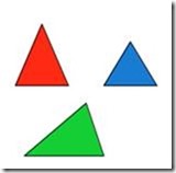
Let’s finish off our basic shape knowledge by learning how to draw a triangle. the triangle function takes 3 sets of XY coordinates, representing the three points of the triangle.
triangle(x1, y1, x2, y2, x3, y3);
Notice the first line of code:
size (200, 200);
The size function sets the screen size of your application (length, width). In this example, the size of the screen is set to 200 by 200 pixels.
6. Make your own creature
Now that we’ve seen how to draw lines, shapes and add color to our drawing, we’re ready to create some drawings of our own! Take a look at the sample creature:
Let’s get on to making your own creature! If you feel comfortable with shape drawing and positioning, feel free to get started. You can also start by changing the colors and positions of the shapes in the sample application until you are happy with the results.
Here are a few fun things you can do to change up the look:
strokeWeight(number)
This will change the thickness of the lines surrounding the creature. Try changing the value and running the application to see the results.
stroke (number)
OR
stroke (RedVal, GreenVal, BlueVal)
The stroke function will change the color of the lines in the drawing. Recall that greyscale shades (from pure white 0 to solid black 255) consist of one argument, and colors 3 values between 0-255 represent the amounts of red, green and blue in the color respectively.


