Outlook
In this chapter, we are going to learn mathematical data manipulations and plotting using NumPy and matplotlib in depth. As we already have seen, NumPy is the core mathematical tool for numerical computing with Python. We first cover how to handle mathematical objects using NumPy. And later, we learn how to produce good looking plots of those mathematical data sets using Matplotlib – another core plotting tool with Python.
Array manipulations in NumPy
In scientific computing, numerical arrays are essential to hold a sequence of numbers. For example, an array can contain:
- values of an experiment/simulation at discrete space and time steps,
- signal recorded by a measurement device, e.g. sound wave,
- pixels of an image, grey-level or colour,
- 3D data measured at different X-Y-Z positions, e.g. MRI scan, etc.
Wait a minute... we already have something like this, i.e., Python lists! Unfortunately, Python lists are not suitable for numerical computing. Let’s first see why.
Python lists vs. NumPy arrays
Python has lists as a built-in data type, e.g.:
>>> x = [1., 2., 3.]
defines a list that contains 3 real numbers and might be viewed as a vector. However, you cannot easily do arithmetic on such lists the way you can with vectors in Matlab, e.g. 2*x does not give [2., 4., 6.] as you might hope:
>>> 2*x
[1.0, 2.0, 3.0, 1.0, 2.0, 3.0]
instead it doubles the length of x, and x+x would give the same thing, which is not what you want in mathematical operations.
Two-dimensional arrays are also a bit clumsy in Python, as they have to be specified as a list of lists, e.g., a 3x2 array with the elements 11,12 in the first row, 21,22 in the second row, 31,32 in the third row would be specified by:
>>> A = [[11, 12], [21, 22], [31, 32]]
Note that indexing always starts with 0 in Python, so we find for example that:
>>> A[0]
[11, 12]

>>> A[1]
[21, 22]

>>> A[1][0]
21
Here A[0] refers to the 0-index element of A, which is itself a list [11, 12]. and A[1][0] can be understood as the 0-index element of A[1] = [21, 22].
You cannot work with A as a matrix, for example to multiply it by a vector, except by writing code that loops over the elements explicitly.
NumPy was developed to make it easy to do the sorts of things we want to do with matrices and vectors, and more generally n-dimensional arrays of real numbers.
For example:
>>> import numpy as np
>>> x = np.array([1., 2., 3.])
>>> x
array([ 1.,  2.,  3.])

>>> 2*x
array([ 2.,  4.,  6.])

>>> np.sqrt(x)
array([ 1.        ,  1.41421356,  1.73205081])
We see that we can multiply by a scalar or take component-wise square roots.
You may find it ugly to have to start NumPy command with np., as necessary here since we imported NumPy as np. Instead you could do:
>>> from numpy import *
and then just use sqrt, for example, and you will get the NumPy version. But in these notes and many Python examples you’ll see, the module is explicitly listed so it is clear where a function is coming from.
Performance comparison
NumPy arrays are more memory efficeint than the usual Python lists in handling
fast numerical operations.
To see the different behavior, we can use timeit module which gives a simple way
to time small bits of Python code. For a more full description,
see https://docs.python.org/2/library/timeit.html.
For instance, timing an operation on a regular Python’s list:
>>> import timeit
>>> setup = '''
... L=range(1000)
... '''
>>> timeit.timeit('[i**2 for i in L]',setup=setup)
51.10083198547363
Using the IPython shell, one can use the convenient %timeit special function instead:
In [22]: L = range(1000)
In [23]: %timeit [i**2 for i in L]
10000 loops, best of 3: 50.8 µs per loop
Notice that this is little bit different from the previous output from a standard Python interpreter, and gives a performance time per loop.
On the contrary, timimg an operation on a NumPy’s array of the same size:
>>> import timeit  # not needed if imported already
>>> setup = '''
... import numpy as np
... a = np.arange(1000)
... '''
>>> timeit.timeit('a**2',setup=setup)
0.8447329998016357
As before, if using the IPython shell:
In [20]: a = arange(1000)
In [21]: %timeit a**2
The slowest run took 8940.42 times longer than the fastest. This could mean that an intermediate result is being cached
1000000 loops, best of 3: 861 ns per loop
Again, this is a time it took per loop.
Creating NumPy data arrays
We looked at a brief example of initializing a NumPy array in the above, where individual items are given explicitly as inputs. In practice, however, we would want to avoid adding items one by one. We can instead use as follows.
Evenly spaced values:
>>> import numpy as np
>>> a = np.arange(10) # np.arange(n) provides indices from 0 to n-1
>>> a
array([0, 1, 2, 3, 4, 5, 6, 7, 8, 9])
>>> b = np.arange(1., 9., 2) # syntax : start, end, step
>>> b
array([ 1.,  3.,  5.,  7.])
or by specifying the number of points:
>>> c = np.linspace(0, 1, 6)
>>> c
array([ 0. ,  0.2,  0.4,  0.6,  0.8,  1. ])
>>> d = np.linspace(0, 1, 5, endpoint=False)
>>> d
array([ 0. ,  0.2,  0.4,  0.6,  0.8])
To specifically initialize a real type array, you can do:
>>> a = np.arange(10, dtype=np.float) # same as a = np.arange(10, dtype=np.float64)
Otherwise, the default setup is integer array:
>>> a = np.arange(10) # same as a = np.arange(10, dtype = np.int)
Constructors for common arrays:
>>> a = np.ones((3,3))
>>> a
array([[ 1.,  1.,  1.],
       [ 1.,  1.,  1.],
       [ 1.,  1.,  1.]])
>>> a.dtype
dtype('float64')
>>> b = np.ones(5, dtype=np.int)
>>> b
array([1, 1, 1, 1, 1])
>>> c = np.zeros((2,2))
>>> c
array([[ 0.,  0.],
       [ 0.,  0.]])
>>> d = np.eye(3)
>>> d
array([[ 1.,  0.,  0.],
       [ 0.,  1.,  0.],
       [ 0.,  0.,  1.]])
NumPy arrays indexing
The items of an array can be accessed the same way as other Python sequences (list, tuple):
>>> a = np.arange(10)
>>> a
array([0, 1, 2, 3, 4, 5, 6, 7, 8, 9])
>>> b = a[0], a[2], a[-1]
>>> b
(0, 2, 9)
>>> type(b)
tuple
For a multidimensional array a, indexes are tuples of integers,
that is, for a 3D array, a[(i,j,k)], or simply a[i,j,k]:
>>> a = np.diag(np.arange(5))
>>> a
array([[0, 0, 0, 0, 0],
       [0, 1, 0, 0, 0],
       [0, 0, 2, 0, 0],
       [0, 0, 0, 3, 0],
       [0, 0, 0, 0, 4]])
>>> a[1,1]
1
>>> a[2,1] = 10 # third line (or row), second column
>>> a
array([[ 0,  0,  0,  0,  0],
       [ 0,  1,  0,  0,  0],
       [ 0, 10,  2,  0,  0],
       [ 0,  0,  0,  3,  0],
       [ 0,  0,  0,  0,  4]])
>>> a[2]   # this is the same as a[2,:]
array([ 0, 10,  2,  0,  0])
Note that:
- In 2D, the first dimension corresponds to lines (i.e., rows), the second to columns.
- for an array a with more than one dimension,
a[i]is interpreted asa[i,:].
NumPy array slicing
Like indexing, it’s similar to Python sequences slicing:
>>> a = np.arange(10)
>>> a
array([0, 1, 2, 3, 4, 5, 6, 7, 8, 9])
>>> a[2:9:3] # [start:end:step]
array([2, 5, 8])
Note that the last index is not included!:
>>> a[:4]
array([0, 1, 2, 3])
start:end:step is a slice object which represents the set of indexes range(start, end, step).
A slice can be explicitly created:
>>> sl = slice(1, 9, 2)
>>> a = np.arange(10)
>>> b = 2*a + 1
>>> a, b
(array([0, 1, 2, 3, 4, 5, 6, 7, 8, 9]), array([ 1,  3,  5,  7,  9, 11, 13, 15, 17, 19]))
>>> a[sl], b[sl]
(array([1, 3, 5, 7]), array([ 3,  7, 11, 15]))
All three slice components are not required: by default, start is 0, end is the last and step is 1:
>>> a[1:3]
array([1, 2])
>>> a[::2]
array([0, 2, 4, 6, 8])
>>> a[3:]
array([3, 4, 5, 6, 7, 8, 9])
- What is the difference between
a[0:1]anda[0::1]?
Of course, it works with multidimensional arrays:
>>> a = np.eye(5)
>>> a
array([[ 1.,  0.,  0.,  0.,  0.],
       [ 0.,  1.,  0.,  0.,  0.],
       [ 0.,  0.,  1.,  0.,  0.],
       [ 0.,  0.,  0.,  1.,  0.],
       [ 0.,  0.,  0.,  0.,  1.]])
>>> a[2:4,:3] #3rd and 4th lines, 3 first columns
array([[ 0.,  0.,  1.],
       [ 0.,  0.,  0.]])
All elements specified by a slice can be easily modified:
>>> a[:3,:3] = 4
>>> a
array([[ 4.,  4.,  4.,  0.,  0.],
       [ 4.,  4.,  4.,  0.,  0.],
       [ 4.,  4.,  4.,  0.,  0.],
       [ 0.,  0.,  0.,  1.,  0.],
       [ 0.,  0.,  0.,  0.,  1.]])
A small illustrated summary of NumPy indexing and slicing:
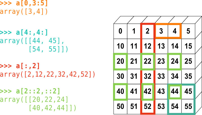
Figure 1: NumPy array indexing.
You can also combine assignment and slicing:
>>> a = np.arange(10)
>>> a[5:] = 10
>>> a
array([ 0,  1,  2,  3,  4, 10, 10, 10, 10, 10])
>>> b = np.arange(5)
>>> a[5:] = b[::-1]
>>> a
array([0, 1, 2, 3, 4, 4, 3, 2, 1, 0])
Copies and views
A slicing operation creates a view on the original array, which is just a way of accessing array data. Thus the original array is not copied in memory. You can use np.may_share_memory() to check if two arrays share the same memory block. Note, however, that this uses heuristics and may give you false positives.
When modifying the view, the original array is modified as well:
>>> a = np.arange(10)
>>> a
array([0, 1, 2, 3, 4, 5, 6, 7, 8, 9])
>>> b = a[::2]
>>> b
array([0, 2, 4, 6, 8])
>>> np.may_share_memory(a, b)
True
>>> b[0] = 12
>>> b
array([12,  2,  4,  6,  8])
>>> a   # (!)
array([12,  1,  2,  3,  4,  5,  6,  7,  8,  9])

>>> id(a[0])
4491149720
>>> id(b[0])
4491149720

>>> id(a)
4584290864
>>> id(b)
4584290304

>>> a = np.arange(10)
>>> c = a[::2].copy()  # force a copy
>>> c[0] = 12
>>> a
array([0, 1, 2, 3, 4, 5, 6, 7, 8, 9])

>>> np.may_share_memory(a, c)
False
Exercise: Extend the above example and use for n in
range(len(b)): to write a short for-loop that checks
if the memory addresses of elements of b are the same as
those of a[::2]. Repeat the same to check c and a.
Component-wise operations
One thing to watch out for if you are used to Matlab notations: In Matlab
some operations (such as sqrt, sin, cos, exp, etc) can be applied to vectors
or matrices and will automatically be applied component-wise. Other
operations like * and / (multiplication and division) attempt to do things
in terms of linear algebra, and so in Matlab, A*B gives the matrix product
and only makes sense if the number of columns of A agrees with the number of
rows of B. If you want a component-wise product of A and B you must use .*
instead, that is, with a period . before the *.
In NumPy, * and / are applied component-wise, like any other operation. To
get a matrix-product you must use dot:
>>> A = np.array([[1,2], [3,4]])
>>> B = np.array([[5,0], [0,7]])
>>> A
array([[1, 2],
       [3, 4]])
>>> B
array([[5, 0],
       [0, 7]])

>>> A*B          # this will not give a matrix-product, but a component-wise product
array([[ 5,  0],
       [ 0, 28]])

>>> np.dot(A,B)  # this is the expected matrix multiplication!
array([[ 5, 14],
       [15, 28]])

>>> np.dot(B,A) # this should be different from np.dot(A,B)!
array([[ 5, 10],
       [21, 28]])
Many other linear algebra tools can be found in NumPy. For example, to
solve a linear system Ax = b using Gaussian Elimination, we can do:
>>> A
array([[1, 2],
       [3, 4]])

>>> b = np.array([2,3])
>>> x = np.linalg.solve(A,b)

>>> x
array([-1. ,  1.5])
To find the eigenvalues and eigenvectors of A:
>>> evals, evecs = np.linalg.eig(A)

>>> evals
array([-0.37228132,  5.37228132])

>>> evecs
array([[-0.82456484, -0.41597356],
       [ 0.56576746, -0.90937671]])
Note: You may be tempted to use the variable name lambda for the eigenvalues of a matrix, but this isn’t allowed in Python because lambda is a keyword of the language, see Lambda functions.
Basic reductions of NumPy arrays
To compute sums:
>>> x = np.array([1, 2, 3, 4])
>>> np.sum(x)
10
>>> x.sum()
10
Sum by rows and by columns:
>>> x = np.array([[1, 2], [3, 4]])
>>> x
array([[1, 2],
       [3, 4]])
>>> x.sum(axis=0)   # columns (first dimension)
array([4, 6])
>>> x[:, 0].sum(), x[:, 1].sum()
(4, 6)
>>> x.sum(axis=1)   # rows (second dimension)
array([3, 7])
>>> x[0, :].sum(), x[1, :].sum()
(3, 7)
Same idea in higher dimensions:
>>> x = np.array([ [[1,2],[3,4]], [[5,6],[7,8]] ] )
>>> x
array([[[1, 2],
        [3, 4]],

       [[5, 6],
        [7, 8]]])
>>> x.sum(axis = 0)
array([[ 6,  8],
       [10, 12]])
>>> x.sum(axis = 1)
array([[ 4,  6],
       [12, 14]])
>>> x.sum(axis = 2)
array([[ 3,  7],
       [11, 15]])
To obtain extrema:
>>> x = np.array([1, 3, 2])
>>> x.min()
1
>>> x.max()
3

>>> x.argmin()  # index of minimum
0
>>> x.argmax()  # index of maximum
1
Logical operations:
>>> np.all([True, True, False])
False
>>> np.any([True, True, False])
True
A few examples in statistics:
>>> x = np.array([1, 2, 3, 1])
>>> y = np.array([[1, 2, 3], [5, 6, 1]])
>>> x.mean()
1.75
>>> np.median(x)
1.5
>>> np.median(y, axis=-1) # last axis
array([ 2.,  5.])

>>> x.std()          # full population standard dev.
0.82915619758884995
Loading data files
Text files
Consider an example: populations.txt:
To load populations.txt:
>>> data = np.loadtxt('./codes/populations.txt')
>>> data
array([[  1900.,  30000.,   4000.,  48300.],
       [  1901.,  47200.,   6100.,  48200.],
       [  1902.,  70200.,   9800.,  41500.],
...
To save it to another name, pop2.txt:
>>> np.savetxt('pop2.txt', data)
>>> data2 = np.loadtxt('pop2.txt')
Other well-known file formats
HDF5: h5py, PyTables
Note
As an example, we will study how to read FLASH’s HDF5 data example in Labels, titles, grids, overplots, legends and Advanced plots – 2D, 3D plots, subplots and more
Other types of file formats that Python can open and read include:
- NetCDF: scipy.io.netcdf_file, netcdf4-python, ...
- Matlab: scipy.io.loadmat, scipy.io.savemat
- IDL: scipy.io.readsav