[7] Numerical Approximations: Euler’s Method¶

In this section, we learn how to solve DEs computationally, or in other words, by writing a computer code to solve DEs numerically.
Many practical applications using mathematical modelings with DEs (ODEs and PDEs) often do not have analytical solutions. This means that we do not know how to solve those problems in practice.
The methods and examples we learned so far are indeed only a fractional part of DEs in which simple analytical ways are available to solve them.
When analytical theories/methods are not avialble, we then need to rely on computer models to study such general, and more challenging DEs.
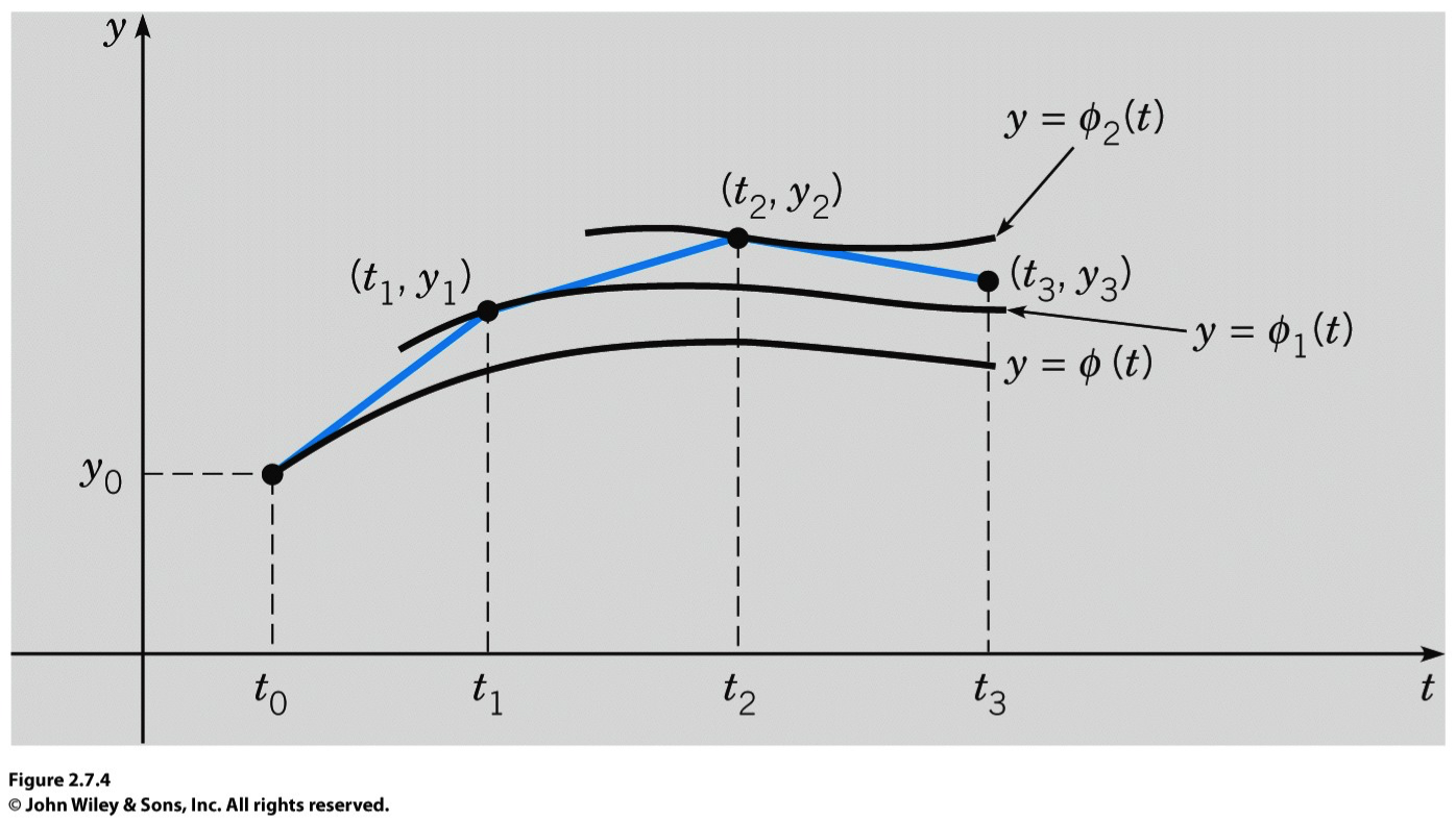
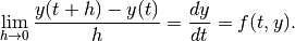
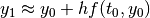
One easy way, due to Euler in about 1768, is based on using tangent lines of the DEs, and the method is called the Euler method (or the tangent line method). To be precise, the method we are going to learn is called the Forward Euler Method in order to represent the discrete approximation of the method is forward in time. That is to say, by considering the definition of derivatives, we see that, for $y'=f(t,y)$ ,

$\lim_{h\to 0} \frac{y(t+h) - y(t)}{h} = \frac{dy}{dt} = f(t,y).$
If we choose $h$ very small then we have

(1) $\frac{y(t+h) - y(t)}{h} \approx \frac{dy}{dt} = f(t,y).$
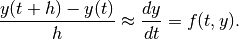
This is called the forward differencing approximation of $\frac{dy}{dt}$ , whereas the backward differencing approximation can be similarly written as

$\frac{y(t) - y(t-h)}{h} \approx \frac{dy}{dt} = f(t,y).$

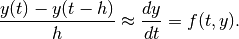
The (forward) Euler’s Method for ODEs

Given the IVP:

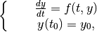
$\begin{equation} \left \{ \begin{array}{ccc} && \frac{dy}{dt} = f(t,y)\nonumber \\ && y(t_0) = y_0, \end{array} \right. \end{equation}$

The Euler method takes the following steps:

Choose the initial point $(t_0,y_0)$ of the IVP.
Introduce a discrete notation $t_1$ to write $t_0 + h$ , and in general,

$t_n = t_0 + n h.$
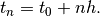
Introduce another discrete notation $y_n$ to write

$y_n = y(t_n) = y(t_0 + n h).$
Then Eq. (1) can be written as a discrete difference equation:

$\frac{y_{1} - y_0}{h} \approx f(t_0,y_0),$

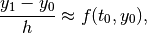
or, equivalently,

$y_1 \approx y_0 + h f(t_0,y_0)$
Assume $h$ is chosen very small enough so that we approximately write

$y_1 = y_0 + h f(t_0,y_0),$

and in the similar way, we successively obtain the $(n+1)$ th term,

$y_{n+1} = y_{n} + h f(t_{n},y_n).$

Examples 1 and 2:¶

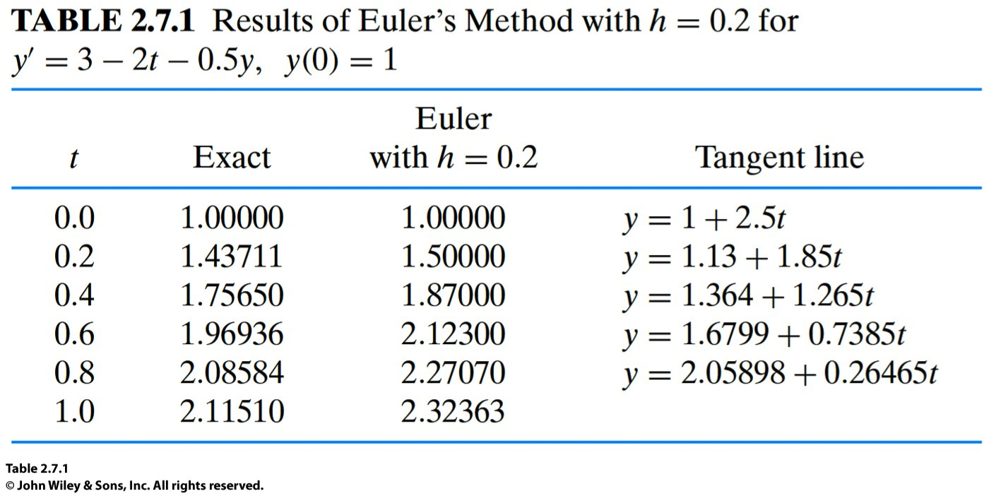
Solve the IVP

$\frac{dy}{dt} = 3 - 2t - 0.5y, y(0) = 1,$

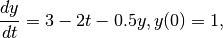
using the Forward Euler method. Note that using the integrating factor $e^{0.5t}$ we can obtain the exact solution

$y = \phi(t) = 14 - 4t - 13 e^{-0.5t}.$

An example Matlab code: Click to download the sample code ForwardEuler.m

% --------------------------------------------%
%      The Forward Euler Method for ODEs      %
%         Written by Prof. Dongwook Lee       %
%                AMS 20/20A                   %
% --------------------------------------------%


% ---------------------------------------------%
% Example 1:                                   %
% * dy/dt = f(t,y) = 3 - 2t - 0.5y             %
% * y(0) = 1                                   %
% ---------------------------------------------%

% [0] clear any previously defined values and
%     figures
clear all;
clf;

% [1] Set initial condition ====================
y0 = 1;



% [2] Set h ====================================
h = .25;



% [3] Set f(t,y) ===============================
f = inline('3 - 2*t - 0.5*y','t','y');



% [3] Temporal Evolution of ODE ================
% [3a] Set your clock to be zero initially
t = 0;

% [3b] Set your maximum timestep
n_step = 100;

% [3c] Set your maximum time based on the 
%      maximum timestep
t_max = 10;
n_max = 1000000;

% [3b] Temporal evolution of ODE until t=t_max
% Set your current y value y_n to be 
% the initial value to begin with
y = y0;

% Provide 1D arrays for solutions of length n_step
y_soln = zeros(n_step,1);
t_soln = zeros(n_step,1);


n = 1;
y_soln(n) = y0;

while (t<=t_max) & (n <= n_max);
    %for n=1:n_max;

        % Forward difference approximation
        y_new = y + h * f(t,y);
        
        % Update your clock
        t = t + h;
        n = n + 1;
        
        % Update your current value of y
        y = y_new;
        
        % Store your time and new solutions
        % in arrays for plot
        y_soln(n) = y;
        t_soln(n) = t;
    %end
    
end



% [4] Plot your numerical solution =============    
figure(1)
plot(t_soln(1:n), y_soln(1:n), 'r*')

% [5] Exact solution
y_exact = inline('14 - 4*t - 13*exp(-0.5*t)','t');

% [6] Overplot exact solution
hold on;
plot(t_soln(1:n), y_exact(t_soln(1:n)),'b');
grid on;

Questions

Study and understand the code, and run it.
Modify the time step size $h$ by increasing or decreasing within the stability range of

$0 \le h \le 4.$

What happens when you increase/decrease your timestep $h$ ?
Modify the time step size $h$ by increasing more than the stability range so that

$h > 4.$

What happens when your timestep $h$ is bigger than the stability limit 4?
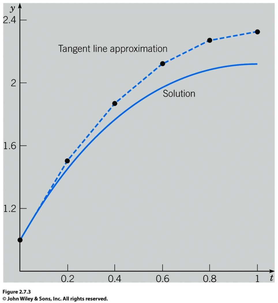
The current code implements to exit the temporal evolution based on the maximum timestep, e.g., n_step. Modify the exit condition so that the code stops when t=t_max, where t_max is any arbitrary time which is not necessarily a multiple of n_step as in the current implementation. (hint: use while loop instead of using for loop.)
Check if you can reproduce the numbers in Table 2.7.1 and Table 2.7.2.

Note

We do not learn how to obtain a stability limit for timestep $h$ in this class. Such topics are covered in more advanced numerical ODE/PDE classes (e.g., AMS 213B).
For this problem, as long as you keep the time step size $h$ to satisfy the stability bound,

$0 \le h \le 4,$

the numerical solutions of the Forward Euler method are stable.

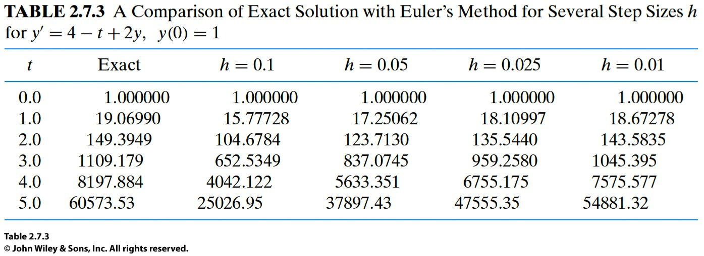
Example 3:¶

Solve the IVP

$\frac{dy}{dt} = 4 - t + 2y, y(0) = 1,$

using the forward Euler method.

Questions

Find the exact solution.
Modify the code in Examples 1 and 2 to solve this problem.
Repeat the steps in Example 1 and 2 and see if the solutions converge by visually inspecting the departure between the numerical and exact solutions, in particular, for large $t$ .

Note

For this problem, the mathematical stability bound of the time step size $h$ becomes

$-1 \le h \le 0,$

which implies the Forward Euler method always fails to be stable, no matter how $h>0$ is small, for the given ODE.
The unstably divergent solution behaviors are shown in Table 2.7.3, in which the differences between the exact and numerical values at times $t=0,1,2,3,4,5$ are much bigger than Examples 1 and 2, for all choices of $h$ .
In this situation, one has to use a different numerical method, such as the backward Euler method (harder than using the forward Euler method in general), in order to stably solve the problem numerically.

Table Of Contents

Previous topic

This Page

[7] Numerical Approximations: Euler’s Method¶

Examples 1 and 2:¶

Example 3:¶