Homework 1 (Due 6 pm, Friday, Apr 8, 2016)
Please submit your homework to your git repo by 6 pm, Fri, Apr 8 2016.
Setup an account from Bitbucket and clone the course repo from the remote Bitbucket repository to your local machine (see the sections in Git Version Control System – Managing Your Coursework).
- Generate and edit a file named
bio.txtwhich includes the following information:
- name, your major, email
- shool year
- research interests
- advisor’s name (if any)
- experience in ODEs and PDEs: (1. a lot, 2. somewhat, 3. none)
- experience in numerical/computational ODEs and PDEs: (1. a lot, 2. somewhat, 3. none)
- experience with MATLAB (1. a lot, 2. somewhat, 3. none)
- do you have MATLAB installed on your local machine? (yes/no)
- if the previous answer is no, do you have an access to a machine that has MATLAB installed? (yes/no)
Check-in (or make a commit)
bio.txtwith a comment:“my first check in to my own repo on mm/dd/yy as part of homework 1”.
After a successful check-in of
bio.txt, modify it by adding a new line on your OS and computer:
- types of OS and machine for the class
- Check-in the updated
bio.txtto the repo again.
- Generate and edit a file named
Modify the example MATLAB code in Example: the Euler’s Methods to solve the IVP using the forward Euler’s method:
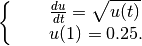
Note that this has a unique exact solution
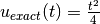 over
over ![[1,\infty]](../_images/math/d3d6715dc65c12b6258afe9af21a338b55e57fff.png) .
Please evolve your numerical solution until the maximum time
.
Please evolve your numerical solution until the maximum time  is reached using
four different time step sizes,
is reached using
four different time step sizes,  . Your grid discretization of
  over
over
![[1,t_{max}]](../_images/math/7ecb8d4da6cf349fe4da166a6f532102ffaa1eaf.png) will be such that
will be such that  , and
, and
 .
.Plot each of the four cases over
![[1,t_{max}] = [1, 5]](../_images/math/52af5c9d9710ad944deedc794a9eefe03e9b282d.png) along with the exact solution.
along with the exact solution.Measure the
 error
error  defined by
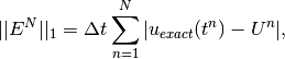
where
 is given by
  .
Plot the error convergence rates by plotting
.
Plot the error convergence rates by plotting  versus in log-log scales (use MATLAB’s
 loglogcommand).