Andriy Mandyev - CMPS 161 Computer Visualization and Computer Graphics – Winter 2010
The goal of this program is to provide the user with a set of tools for flow visualization. The user is able to generate a 2 dimensional vector representing the flow that he wants to study and then apply a variety of visualization methods on this field.
The program starts with the vector field initialized to zero, so to flow is inexistent. The user can specify the by creating one or several reference vectors inside the field. This is done by simply clicking on a position where the vector will be located and then dragging the mouse to specify its norm. After a new reference vector is added, the program recalculates the values of the field using the Shepard’s method.
Furthermore a predefined field can be loaded, so the user is not forced to recreate one manually each time.
Once the vector field is created, the user will have the possibility to visualize the flow using one of the following techniques:
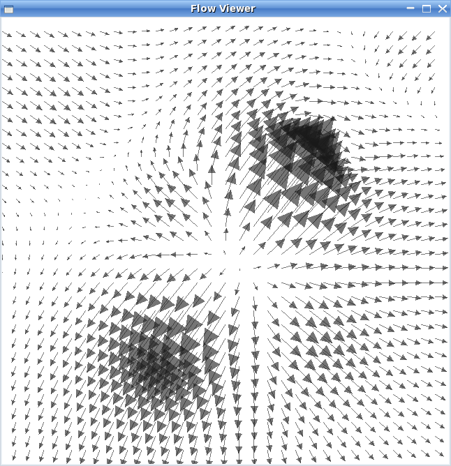
1. We can simply represent each vector with an arrow on a uniform grid. However, if the grid is too dense compared to the norm of the vectors, it can become very difficult to observe anything.
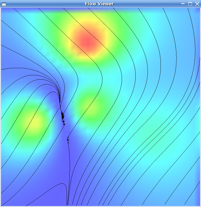
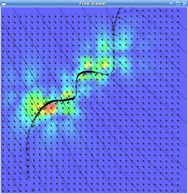
2. A good alternative to this is to normalize the vectors before display, so that they don’t take up the space of their neighbors. Although we lose the information about the intensity of the flow, the direction becomes more visible. In order to keep track of the velocity, we can use color mapping. On the picture below, the colors represent the pressure of the flow at a given point. Since the pressure is proportional to the velocity squared, it serves as a good indicator. Blue represents low values and red the highest ones.

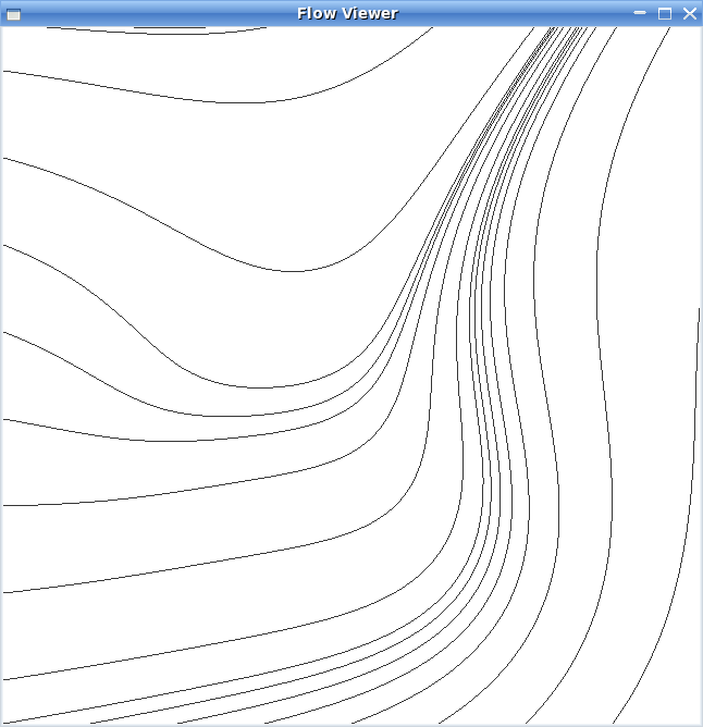
3. The clearest way to observe a flow is to use streamlines. The streamlines are calculated using Euler’s integration and a window borders as initial points. Although this method is less precise than Runge-Kutta, we chose to implement it because it is faster.
4. The problem with streamlines is that they are discrete, which can lead to big chunks of blank with nothing to observe. The way we deal with this problem is by plotting a lot of streamlines with the initial points very close to each other. Different colors are used for each streamlines in order to differentiate them. This creates the effect of a continuous flow where we can observe most parts of the field.r
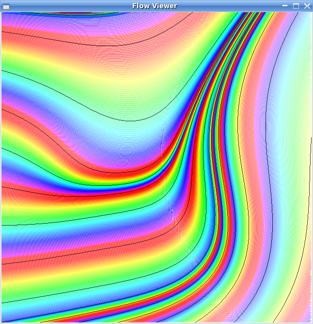
5. Yet another way to use color mapping is to represent the turbulence of the flow.
Most of the actions can be performed via the context menu triggered by the right mouse button, however there are some keyboard shortcuts:
‘a’ – switches between different arrow representations.
‘b’ - switches between different uses of color mapping.
‘g’ – show/hide the grid.
‘v’ – show/hide the reference vectors.
‘r’ – reset all parameters do default values.
Escape – exit the program.
To create a new reference vector left click and drag.