CMPS 161 - Final Project Winter 2008
~ Streamlines Visualization ~
Andres Sopena Perez (asopenap@ucsc.edu)

Platform:
- Ubuntu Linux 7.10
- GCC/g++, OpenGL, FLTK
Study of alternative
simple and
fast ways of visualizing streamline fields that do not involve
integration
methods such as the Euler integration method or Runge-Kutta 4.
Two different strategies have been followed:
CompilationTwo different strategies have been followed:
- Strategy 1: Convert the corresponding vector field into a scalar field and use scalar field visualization techniques.
- Strategy 2: Use the already computed vector field grid vertices as the successive steps of the line integration to obtain a fast representation.
- Introduction: Vector fields.
- Vector field visualization: streamlines and their associated problems.
- Strategy 1: Integration simplification.
- Strategy 2: Converting to scalar field.
>make
Execution
>./skl
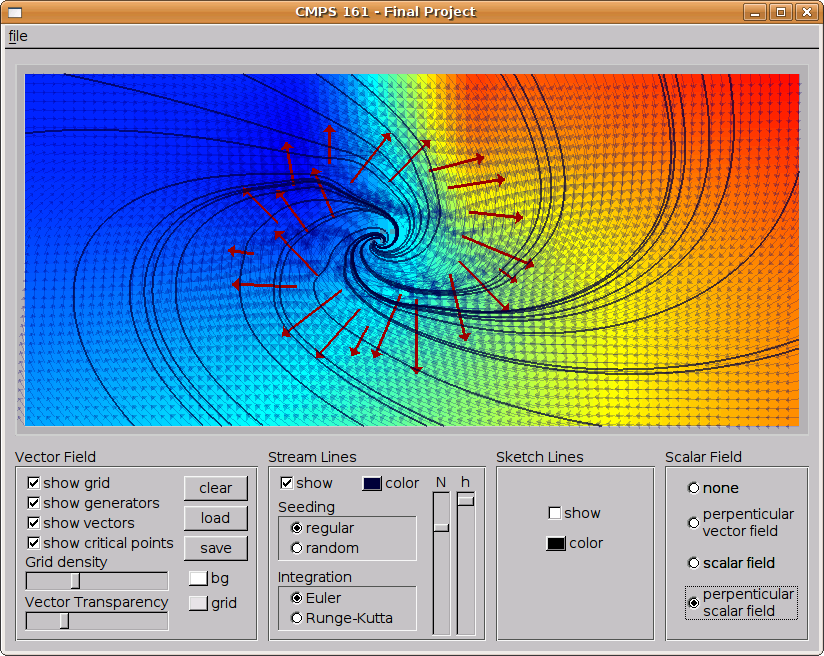
Brief User Guide
The core of the
project is the visualization application developed to
test the different approaches. Its use is fairly straightforward:
To create a new vector field
The application starts with an empty vector field (one in which all vectors are null).
Use the load button to load a new vector field from disk (file extension *.161) or create your own vector field by clicking and dragging on the field area.
Each time you click and drag a new generator vector (red color) will be created. The vectors of the vector field are calculated using Shepherds Interpolation on the generator vectors.
To clear the field again, click on the clear buttom.
To see the field covering the whole window click on the right button of the mouse. To go back to the original size, click on it again.
Vector field
The options in the Vector field box allow the user to activate and deactivate the elements to show. The grid density slider allows to change the size of the cell.
Stream Lines
Check Show to see the stream lines of the current field.
h - step size [0.1 , 1]
N - number of seeds
It is also possible to change the seeding method and the integration method.
Sketch Lines
To see the results of the strategy 1, click on Show.
Scalar Field
To see the different options tried for strategy 2, click on the desired option.
Introduction: Vector Fields |
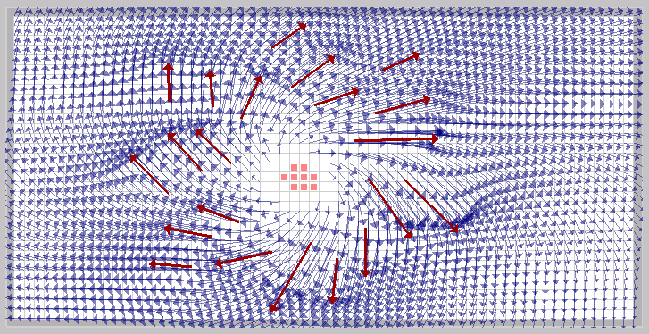
The goal of this project is to study methods to visualize vector fields. A vector field is a collection of data related to a particular physical environment. If you describe a physical property for each point in space the result is a field. If that property, such as temperature, is defined by a scalar, the result is a scalar field. If the property is defined by a vector the result is a vector field. An example of vector field is one that describes the wind velocity over a terrain.
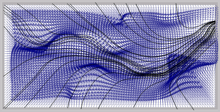
A common way of visualizing a scalar field is as a grid in which each vertex has an associated vector:
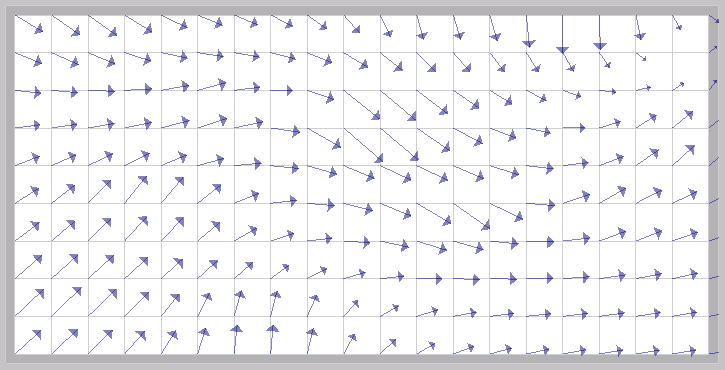
This visualization
method is known as the Hedgehog Plot. In general, it is only
satisfactory for small grids with little
information. As soon as the amount of information to visualize starts
to grow, the image becomes confusing and it is difficult to determine
the direction of the arrows:
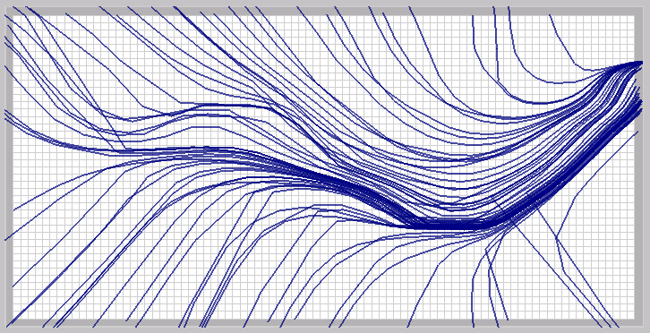
Vector field visualization: streamlines |
To solve this problem, usually vector fields are visualized as stream lines, which are lines drawn following the flow of the arrows:
This makes the image
much easier to understand. For instance, if the vector field shows the
wind velocity in each region over a terrain, the streamlines allows us
to
have an intuitive understanding of the wind direction in each point. Of
course, this is even more clear if only the streamlines are drawn:

The problem of this
visualization technique is that to draw each line it is necessary to
integrate the vectors along the path, and it is therefore
computationally expensive. Two usual integration methods are used,
Euler and Runge-Kutta 4. Euler is faster but Runge-Kutta provides
better
results.
For instance, the last image of the previous section:
has been computed with h = 0.1. However, if we increase h to 1, the above mentioned problems start to appear:
Runge-Kutta is far less prone to these problems, but at the cost of computing 4 interpolated vectors instead of one, which means that it is also time consuming.
In the next sections, we are going to see the alternative methods that have been studied for this project.
Strategy 1: Integration simplification. |
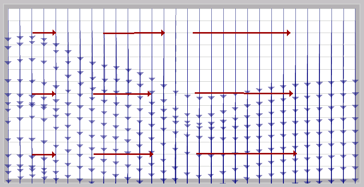
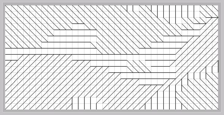
The main problem of Euler and RK4, as we have seen, is the necessity of having to interpolate the corresponding vectors for all steps in the line path. The following strategy tries to address that problem. The idea consists in jumping from vertex to vertex of a precomputed vector grid. In this way, it is not necessary to calculate the new vector in each step since we know the vector values at the vertices. The result is necessarily going to be much less precise that the traditional integration, because starting from one vertex there are only 8 possible directions to follow (the 8 adjacent vertices):
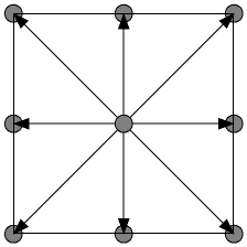
However, the
computation can be faster since there is no necessity to integrate
(always that we have a precomputed grid, of course) and it is necessary
to read the vector angle to know the following point.
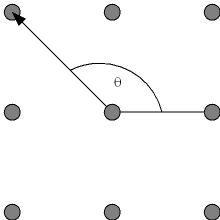
Thus, constructing the line is basically a process of checking the angle select new vertex from the 8 adjacent ones and repeat the process until the line is complete.
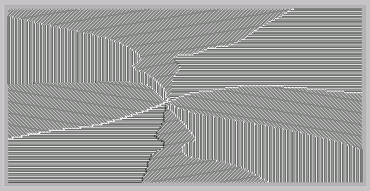
The results, for this technique have been unexpected. When the cell size is big, the image turns out to be not very useful:
Thus, constructing the line is basically a process of checking the angle select new vertex from the 8 adjacent ones and repeat the process until the line is complete.
The results, for this technique have been unexpected. When the cell size is big, the image turns out to be not very useful:
The flow it is very
difficult to determine, although this could be expected since the cell
size roughly correspons to what h is in Euler Integration
method.
When the cell size is small however, clear patterns of direction appear:
When the cell size is small however, clear patterns of direction appear:
The lack of precision
in the technique makes it easy to identify regions of similar flow.
This can be particularly useful when dealing with critical points.
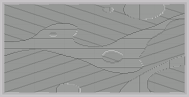
Critical points are those in which the corresponding vectors are equal to zero. That is, there is no flow through them. They are probably the points of more interest in the image. An example of one of them is this:
Critical points are those in which the corresponding vectors are equal to zero. That is, there is no flow through them. They are probably the points of more interest in the image. An example of one of them is this:
This one is called
spiral source, and the critical points are inside the cells marked with
red. A requirement to any visualization technique is that it shows
clearly where the critical points are.
With the new technique, the critical point shown above is displayed as:
With the new technique, the critical point shown above is displayed as:
As it can be seen,
this technique could be useful to determine singular points by means of
line patterns.
The following technique is based on the concept that the visualization of scalar fields is generally easier and faster than the visualization of vector fields. The strategy in this case is therefore to conver the vector field to a scalar field and try to get contour lines (lines that joint points with the same scalar value) that are equivalent to streamlines.
To try to do this, the following steps have been followed:
Strategy 2: Converting to scalar field. |
The following technique is based on the concept that the visualization of scalar fields is generally easier and faster than the visualization of vector fields. The strategy in this case is therefore to conver the vector field to a scalar field and try to get contour lines (lines that joint points with the same scalar value) that are equivalent to streamlines.
To try to do this, the following steps have been followed:
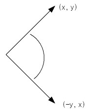
- find the perpenticular vector field to the current vector field. The perpenticular vector field is that one in which each vector is the same but perpenticular to the one in the original field.
This is very easy
and fast to manage since the perpenticular vector to (x, y) is
(-y, x), and therefore it is necessary only to swap values and
change the sign of one of them.
- find the scalar field that corresponds to the perpenticular vector field. This has to be done as fast as possible because it is the step more computationally expensive. To do it the scalar value of each vertex of the grid is calculated according to the scalar value of the vertex just below it. To start with a value the first vertex is set arbitrarily to 0 and then all the rest of the vertices are calculated according to it.
To calculate the scalar value of a vertex (x, y): Sxy = [SIN ANGLEx,y-1 ] * Sx,y-1
- Finally, the contour lines of the scalar field are drawn.
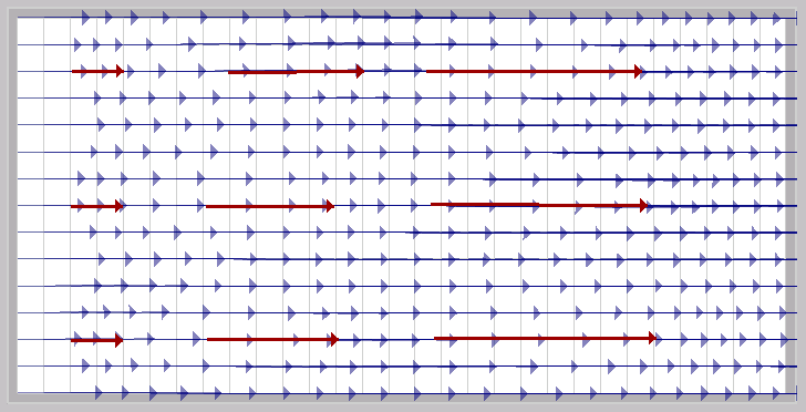
Original vector field
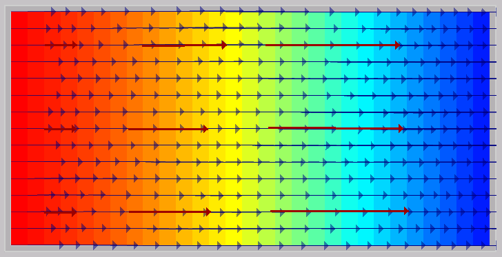
Equivalent scalar field:
Perpenticular vector field: