
The program that I have written for my final graphics assignment is a 3D Pool Game simulation. The main relevance of my assignment to the course is the implementation of physically based modeling. More specifically, I have implemented the motion of the billiard balls based on real life physics equations. The implementation of those equations seemed to have come out well in this program, for the collisions actually act realistic.
Unfortunately, I was not able to completely implement the whole game. In fact, to be quite honest, I have barely had any time this quarter to do this program and in turn I did not get to implement some of the easier things such as even having pockets! My pool table is also on a green rectangle. The part of the program that I have done, however, is material that I have newly learned this quarter and I am hoping that this will be taken note of when my grade on this project is being decided. This program turned out to be much harder than I imagined but I did still do a lot of work on it.
All of the interaction in the game is done with the mouse. When the program starts, the user can rotate the world view (i.e. the camera) to get a different/better view of the table top by moving the mouse any which way. I have limited the camera rotations to only rotate about the x and z axes though. By holding the third mouse button (right button) down and moving the mouse at the same time, the user can rotate just the pool stick into an orientation that they would like to hit the cue ball with. If they hold the middle mouse button, and simultaneously move the mouse up , a "zoom in" is performed. Likewise, if they do the same but move the mouse down , then a "zoom out" is performed.
If the user clicks mouse button 1 (i.e. the left mouse button), then they toggle the game mode between shooting/aiming. Initially, the game state is set to aiming, so the first time the user clicks the left mouse button in the program it toggles to "shooting" mode. Here is a complete list of the program commands:
I have made this program using GLUT display methods, however, to make it possible for the program to be "full screen" mode I had to include some extra code that facilitates the simultaneous use of FLTK and GLUT. What this means is that when the user starts the program, a small FLTK GUI pops up that asks for the user to specify the screen resolution as well as color depth and frame rate if they want. This code was taken from the first of two resources that I used in this program and I have documented that in the program.
The physics in this program is based exactly on currently known physics equations that
are used in motion. For the motion of a single ball, the equation to move it is simplier than
Newton's Force laws because I do not base motion on time in the program. What this means is
that instead of using Newton's Force law of F = ma where a is an average acceleration,
which is based on a time variable, I use the following simplier equation for single ball motion:
new_Position(A) = old_Position(A) + Velocity(A)
In the above equation, A is denoted as an arbitrary ball, and both Postion(A) and Velocity(A) are 3-dimensional vectors. Implementation of this equation is clearly evident and commented in my UpdateBall() function near the top of the implementation file.Collisions in this game, however, must be dealt with using the precise physics equations that have been defined many years ago. When colliding two balls, where one, two or none of them may be moving, the Conservation of Momentum equation must be followed. Using the Conservation of Momentum , the resulting velocity and direction vectors after the collision are obtained, and then they are applied when the main loop of the program updates all of the ball positions and then redraws the scene. The Conservation of Momentum is as follows:
P = P(A) + P(B) = M(A)V(A) + M(B)V(B)
where P represents the total momentum of the system, P(k) represents the momentum of ball "k", M(k) represents the mass of ball "k", and V(k) represents the velocity of ball "k." One should note that for the above equation, the mass of A or B, written as M(A) or M(B), is a scalar. All of the other parts in the Conservation of Momentum equation are vectors and have x, y, and z components.Keeping that equation in mind, we realize that in a situation where you have two (or more) balls hitting each other, that the momentum before the collision is the same as after it. This yields the following equation for the x-components of a collision where momentum is conserved:
M(A)V(A1x) = M(B)V(B1x) = M(A)V(A2x) + M(B)V(B2x)
The same equation applies for the y and z components of balls A and B by setting up the corresponding components in the equation. One should note that it easy to switch the above equation around to set it up so that it solves the values for the "after collision" velocities. For example, we can set up the equation so that it solves for V(A2x) to try and find the x component of the velocity of ball A after the collision.However, taking this equation even further and making it more useful, one of my resources for this project provided the following equations for simulating the collisions:
V1f = V1i + nc
V2f = V2i - nc
where v1f represents the final velocity of the first object, v1i is the initial velocity of object one, c = n dot (V1i - V2i) / (n dot n) and n = normal unit vector from object 1 to object 2. These equations are implemented in the FixVectors() function of the code.The final physics implementation is the program is the use of friction . Since I am implemeting the Conservation of Momentum equation for collisions, if friction was not present in the program, then the balls would roll forever. So a friction equation has been implemented which simply muliplies the veocities of the balls by a friction factor. That friction factor is a #define'd value that can be increased or decreased to see its effects on the motion.
While friction is constantly applied to all of the balls at all times when they are moving, an additional friction force is also applied when a ball hits any wall. This is done to simulate the ball loosing some energy (hence momentum) when it hits the wall which is what happens in real life. When any ball hits a wall, its velocity is decreased by 5 times the frictional force. After messing with the numbers, I think that 5 times the frictional ammount yields decent results.

While I was not able to implement the scoring part of this project (i.e balls going into pockets) I was able to implement much needed camera work for this project. First of all, when the user hits the cue ball, if the "follow" mode is toggled on then when the cue ball is hit, the camera follows it until it comes to a stop. This works pretty well except for a minor bug of the cue stick not sometimes lining up with the new position of the cue ball.
If the user simply moves the mouse without holding down any mouse button, then the cue stick rotates around the cue ball for aiming. The way I did this is I simply rotate the cue stick around the location of the cue ball.
Other camera movements are being able to zoom in/out of the scene, and being able to translate the viewpoint (camera) around the scene. These actions were implemented using simpe glRotate() and glTranslate() statements in the right places (i.e. for the right matrix stacks.) How to perform these actions is discussed in the USAGE section of this document.
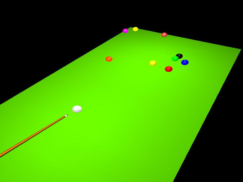
More Screen Shots:
