BME210 Lab 6

Part II

1. I wrote my own code for this before the solution was given:

   cocluster.index <- function (a, b) {
       match <- mismatch <- 0
       for (i in 1:length(a)) {
       apairs <- which(a == a[i])
       bpairs <- which(b == b[i])
       apairs <- apairs[apairs>i]
       bpairs <- bpairs[bpairs>i]
       
       o <- which(apairs %in% bpairs)
       overlap <- length(o)
       match <- match+overlap
       mismatch <- mismatch + length(apairs) + length(bpairs) - 2*overlap
     }
     match / (match+mismatch)
   }

2. centers <- 15
   runs <- 10
   cluster.kmeans <- apply(as.matrix(1:runs), 1,
                           function(x){kmeans(stress.submatrix,centers)$cluster})
   
   cluster.kmeans.cocluster <- NULL
   for(i in 1:(runs-1)) {
     for (j in (i+1):runs) {
       val <- cocluster.index(cluster.kmeans[,i],cluster.kmeans[,j])
       cluster.kmeans.cocluster <- c(cluster.kmeans.cocluster, val)
     }
   }

   
3. 

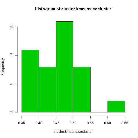
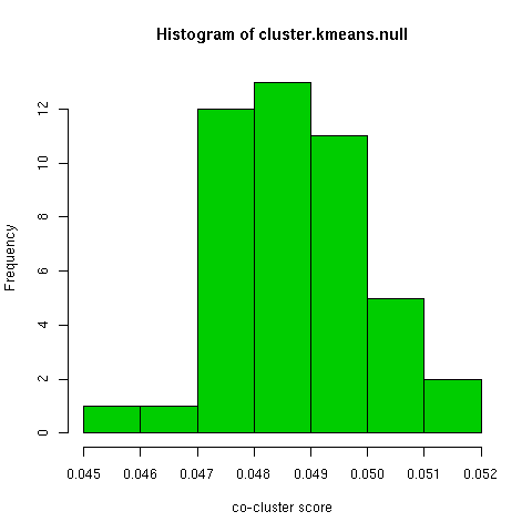
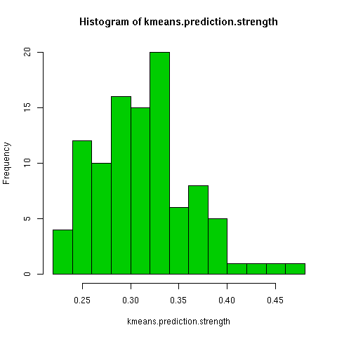
   The kmeans clustering has a wide degree of variability under this measure, about 0.3. When i randomly permuted the first clustering and used the co-cluster measure, the range of scores was much smaller than between all the kmeans clusterings, by about a third. For a more direct comparison with the permuted co-clusters, I looked at just the comparison of the first kmeans clustering with the other 9 kmeans clusterings, and this distribution had very little overlap with the null distribution.

4. By trying kmeans-clustering 10 times on each value of k, for lots of values of k, you could pick the k that gives you the smallest mean cocluster.index value.

Part III

1. I kind of like the methods that I came up with for centroids and assign (aggregate is a really useful function):

   compute.centroids <- function(X, assign) {
     aggregate(X, by=list(Cluster=assign), mean)[,2:(ncol(X)+1)]
   }
   assign.clusters <- function(X, C) {
     apply(X, 1, function (x) {
       which.min(as.matrix(dist(rbind(x,C)))[1,2:(nrow(C)+1)])
     } )
   }
   

2. 
3. 

   The hierarchical clustering seems to have fewer bad outliers, so on the basis of this measure I prefer the hierarchical clustering.

Part IV

1. used the builtin function
2. 

   The best cluster only has 2 genes in it (but four spots):PAE2989 PAE2989 PAE3024 PAE3024. The second best group has 12 genes, the top 10 being: PAE2480 PAE2644 PAE0143 PAE2644 PAE.i262 PAE0143 PAE2480 PAE2659 PAE2659 PAE2693.

3. The most straightforward way would be to use the k or method that gives the best overall average of the silhouette value. Instead of using the average of all s(i), one could punish negative values more by replacing them with the negation of the square or something like that. I didn't like how hierarchical clustering looked with this plot, so I redid it with kmeans and got results that look a lot better. Also, the top scoring clusters are of a more reasonable size.

   

Part V

1. The five FASTA files that I created had some X's in them, so I removed them and ended up with:

   • Cluster 1
   • Cluster 2
   • Cluster 3
   • Cluster 4
   • Cluster 5

2. clust1
   Motif #1: (ATGGCGCATT/AATGCGCCAT)
   Motif #2: (TGAAGAGGGG/CCCCTCTTCA)
   Motif #3: (CGACAAGCTT/AAGCTTGTCG)
   clust2
   Motif #1: (ACCACATTAG/CTAATGTGGT)
   Motif #2: (TAAATGAAAT/ATTTCATTTA)
   Motif #3: (ATTTCATTTA/TAAATGAAAT)
   clust3
   Motif #1: (GGGTTGAAGA/TCTTCAACCC)
   Motif #2: (GGCGTTGAAG/CTTCAACGCC)
   Motif #3: (GCGACGCTTC/GAAGCGTCGC)
   clust4
   Motif #1: (CGGCGTCTTC/GAAGACGCCG)
   Motif #2: (AGCCGCCGCC/GGCGGCGGCT)
   Motif #3: (AGCCGCCGAG/CTCGGCGGCT)
   clust5
   Motif #1: (CGGGGAGGTG/CACCTCCCCG)
   Motif #2: (CGACGAGGTG/CACCTCGTCG)
   Motif #3: (CGGGGAGGTG/CACCTCCCCG)

3. For each cluster, we could divide it into two halves, put each half through BioProspector, and see if we get the same motifs back.