
The majority of genes followed either a decreasing or increasing expression profile throughout the time course. In particular, clusters 1, 2, and 3 decrease throughout the time course, and clusters 9, 10, 11, 12, 13, and 14 increase throughout the time course. The other clusters display more complex behavior. Figure 1 shows clusters and enriched TIGR role categories.
|
Figure 1. SOM clustering of all spotted ORFs. Yellow indicates expression above that at hour 1, blue indicates lower expression. Enrichment for TIGR functional sub-role categories was computed using the standard hyper-geometric method, and some significantly scoring categories are placed by each cluster. |
The chemotaxis and motility genes show a general trend of up regulation throughout the growth curve. These genes were split primarily between two clusters, 9 and 11, and show slightly different expression profiles. In general, genes in cluster 11 show an increase in expression slightly after those in cluster 9, and the separation of chemotaxis and motility genes will be justified, especially when looking at the flagellar operon. Upregulation of chemotaxis and motility during log phase and stationary phase is interesting in that V. cholerae seems to anticipate the need for a new food source, as it enters log-growth.
The proteins for ribosomal synthesis and ribosomal subunits generally fall into two different clusters, that share the general profile of downregulation later in the cell cycle. Downregulation of ribosomes later in the growth curve is sensible, as cells would focus most of their transcriptional energy on growth.
Pathogenesis genes are split amongst nearly all the clusters, and show a wide variety of expression profiles. However, most of the pathogenesis genes return to either hour 1 expression or lower expression in stationary phase.
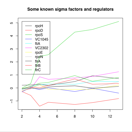
Expression data through a growth curve provides a unique opportunity to examine the exchange of sigma factors in V. cholerae. Figure 2 shows the expression of some known sigma factors and their expression.
 |
 |
 |
Figure 2. Expression of some known sigma factors and regulators. The sigma factors rpoD and rpoS show the greatest fold change in expression, approximately +32-fold and -3-fold respectively. VC2302, an extra-cytoplasmic-function related protein of unknown function or regulons, shows two-fold upregulation. |
| (a) | (b) | (c) |
|---|
Our method of regulon detection finds several regulators for some clusters. However, for successful regulators, most of the ‘+’ and ‘-’ categorizations appear to result from small variance around the mean rather than truly increased or decreased expression. In addition, the method misses several known regulators, and the highly expressed rpoS is not predicted as the regulator of any of the highly up-regulated gene clusters. This all leads to the conclusion that there is much room for improvement is the regulon prediction method. One interesting avenue of exploration would be to introduce a time lag between the increase of a sigma factor and the response of the potentially regulated genes.
|
Table 1. Positive regulator scores by cluster. As described in the methods, each potential regulator was scored against each cluster. Sigma factor rpoE and regulator flrA have high variance to mean ratios, but low overall expression, and score well than other, more significantly expressed sigma factors and regulators. |
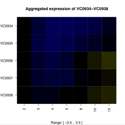
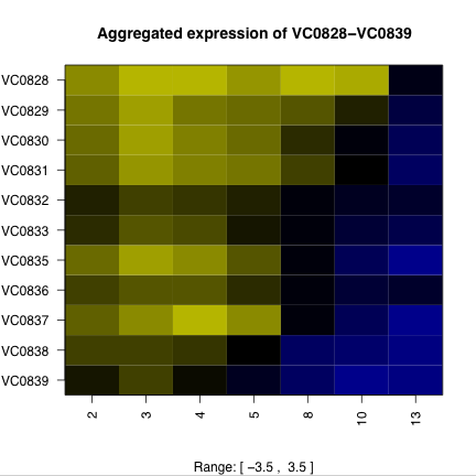
Time course data also provides an opportunity to predict operons and their degradation. Figure 3 shows the expression profiles of some putative operons and surrounding areas of the chromosome. The high degree of structure in the expression of putative operons suggests the possibility of predicting operons purely from expression data. A first attempt would be to calculate the pairwise correlations of neighboring genes, and looking for islands of high correlation.
 (a) |
 (b) |
Figure 3. Putative operons and surrounding chromosome expression. The ORFs of putative operons (a and c) show a distinctive pattern of expression that the surrounding ORFs (b and d) do not exhibit. Operon VC0934-VC0938 (a and b) is on the plus strand and operon VC0839-VC0828 is on the minus strand. Degradation of the mRNA from the 5’ end would explain the expression pattern. |
|---|---|---|
 (c) |
 (d) |
Specific growth conditions of V. cholerae available from Yildiz lab. Lag-phase cells were placed in fresh medium, and grown for 13 hours. Samples were taken at 1, 2, 3, 4, 5, 8, 10, and 13 hours, from two different cultures. RNA was extracted from each sample and then labeled (hour 1 with Cy3, all others with Cy5). Each RNA sample was then divided into two and hybridized to it's own array. Each array was analyzed using GenePix software, and then each image from hours 2 through 13 were superimposed on images of hour 1.
The data was loaded into BioConductor and normalized with print-tip loess. For each ORF, all available M-values were collected across replicates and spots on the chip then averaged. This aggregated data was then clustered using a 4x4 self-organizing map, using Cluster.
A list of potential regulators was generated from the TIGR annotations and literature by F. Yildiz. The likelihood of regulator generating the data from a cluster was calculated as follows: the mean expression of the regulator is calculated, and then each time point is divided into one of the two categories ‘+’ or ‘-’. For each cluster, all the data points under the ‘+’ points are pooled, and the mean and the variance of the data are estimated. The likelihood of the ‘+’ time points is calculated by assuming that they were generated from a normal distribution with a mean and variance of the estimated data. The likelihood for the ‘-’ are calculated similarly. The likelihood of the cluster data given the is then equal the likelihood of the ‘+’ times the likelihood of the ‘-’ data. Finally, this likelihood is divided to the likelihood of the cluster data without splitting the data, and the log is taken to give a log likelihood.